
Selected: Edexcel A Level Maths - Pure Maths
AS & A2 (Whole Course) - All Questions - Casio fx-991EX
Register / Login for More / Subscribe for All Without Ads
AS & A2 (Whole Course) - All Questions - Casio fx-991EX
Register / Login for More / Subscribe for All Without Ads

-
Jun 25 A2
Q S5 Jun 25 A2
Q S5
-
Jun 24 A2
Q S5
Jun 24 A2
Q S5
-
Jan 24 A2
Q S6 ab Jan 24 A2
Q S6 ab
-
Jan 23 A2
Q S5 de
Jan 23 A2
Q S5 de
-
Jun 22 A2
Q S2 Jun 22 A2
Q S2
-
Dec 21 A2
Q S5
Dec 21 A2
Q S5
-
Mar 20 A2
Q S2
Mar 20 A2
Q S2
-
Mar 20 A2
Q S4 c
Mar 20 A2
Q S4 c
-
Jun 19 A2
Q S2
Jun 19 A2
Q S2
-
Jun 19 A2
Q S2
Jun 19 A2
Q S2
-
Jan 19 A2
Q S1 d
Jan 19 A2
Q S1 d
-
Jan 19 A2
Q S4
Jan 19 A2
Q S4
-
Jan 19 A2
Q S5 bcd
Jan 19 A2
Q S5 bcd
-
Jun 18 A2
Q 5 abc
Jun 18 A2
Q 5 abc
-
May 18 A2
Q S3 b
May 18 A2
Q S3 b
-
May 18 A2
Q S5
May 18 A2
Q S5
-
May 17 A2
Q 1 def
May 17 A2
Q 1 def
-
May 17 A2
Q 5 cde
May 17 A2
Q 5 cde
Edexcel 9MA0/03 Jun 2025 A2 Exam Q. S5
 10 marks in 12:00 min.
Vote:
 (0)
(0)
 (0)
(0)
 (0)
(0)
Request * Pop-Up Working * (0)
Request * Pop-Up Working * (0)
Edexcel 9MA0/03 Jun 2024 A2 Exam Q. S5
10 marks in 12:00 min.
Vote:
(0)
(0)
(0)
Request * Pop-Up Working * (0)
Request * Pop-Up Working * (0)

Edexcel 9MA0/03 Jan 2024 A2 Mock Q. S6 ab
5 marks in 6:00 min.
Vote:
(1)
(0)
(0)
Request * Pop-Up Working * (0)
Request * Pop-Up Working * (0)
Edexcel 9MA0/03 Jan 2023 A2 Mock Q. S5 de
5 marks in 6:00 min.
Vote:
(0)
(0)
(0)
Request * Pop-Up Working * (0)
Request * Pop-Up Working * (0)
Edexcel 9MA0/03 Jun 2022 A2 Exam Q. S2
12 marks in 14:24 min.
Vote:
(0)
(0)
(0)
Request * Pop-Up Working * (0)
Request * Pop-Up Working * (0)
Edexcel 9MA0/03 Dec 2021 A2 Mock Q. S5
14 marks in 16:48 min.
Vote:
(0)
(0)
(0)
Request * Pop-Up Working * (0)
Request * Pop-Up Working * (0)
Edexcel 9MA0/03 Mar 2020 A2 Mock Q. S2
11 marks in 13:12 min.
Vote:
(0)
(0)
(0)
Request * Pop-Up Working * (0)
Request * Pop-Up Working * (0)
Edexcel 9MA0/03 Mar 2020 A2 Mock Q. S4 c
3 marks in 3:36 min.
Vote:
(0)
(0)
(0)
Request * Pop-Up Working * (0)
Request * Pop-Up Working * (0)
Edexcel 9MA0/03 Jun 2019 A2 Shadow Exam Q. S2
11 marks in 13:12 min.
Vote:
(0)
(0)
(0)
Request * Pop-Up Working * (0)
Request * Pop-Up Working * (0)
Edexcel 9MA0/03 Jun 2019 A2 Exam Q. S2
11 marks in 13:12 min.
Vote:
(0)
(0)
(0)
Request * Pop-Up Working * (0)
Request * Pop-Up Working * (0)
Edexcel 9MA0/03 Jan 2019 A2 Mock Q. S1 d
2 marks in 2:24 min.
Vote:
(0)
(0)
(0)
Request * Pop-Up Working * (0)
Request * Pop-Up Working * (0)
Edexcel 9MA0/03 Jan 2019 A2 Mock Q. S4
11 marks in 13:12 min.
Vote:
(0)
(0)
(0)
Request * Pop-Up Working * (0)
Request * Pop-Up Working * (0)
Edexcel 9MA0/03 Jan 2019 A2 Mock Q. S5 bcd
6 marks in 7:12 min.
Vote:
(0)
(0)
(0)
Request * Pop-Up Working * (0)
Request * Pop-Up Working * (0)
Edexcel 9MA0/03 Jun 2018 A2 Exam Q. 5 abc
9 marks in 10:48 min.
Vote:
(0)
(0)
(0)
Request * Pop-Up Working * (0)
Request * Pop-Up Working * (0)
Edexcel 9MA0/03 May 2018 A2 Mock Q. S3 b
6 marks in 7:12 min.
Vote:
(0)
(0)
(0)
Request * Pop-Up Working * (0)
Request * Pop-Up Working * (0)
Edexcel 9MA0/03 May 2018 A2 Mock Q. S5
8 marks in 9:36 min.
Vote:
(0)
(0)
(0)
Request * Pop-Up Working * (0)
Request * Pop-Up Working * (0)
Edexcel 9MA0/03 May 2017 A2 Sample Exam Q. 1 def
5 marks in 6:00 min.
Vote:
(0)
(0)
(0)
Request * Pop-Up Working * (0)
Request * Pop-Up Working * (0)
Edexcel 9MA0/03 May 2017 A2 Sample Exam Q. 5 cde
5 marks in 6:00 min.
Vote:
(0)
(0)
(0)
Request * Pop-Up Working * (0)
Request * Pop-Up Working * (0)
-
Jun 23 A2
P3 Q 16
Jun 23 A2
P3 Q 16
-
Jun 22 A2
P3 Q 11
Jun 22 A2
P3 Q 11
-
Jun 22 A2
P3 Q 18
Jun 22 A2
P3 Q 18
-
Nov 21 A2
P3 Q 18
Nov 21 A2
P3 Q 18
-
Nov 20 A2
P3 Q 17
Nov 20 A2
P3 Q 17
-
Jun 19 A2
P3 Q 17
Jun 19 A2
P3 Q 17
-
Jun 18 A2
P3 Q 16
Jun 18 A2
P3 Q 16
-
Jun 17 A2
P3 Q 13
Jun 17 A2
P3 Q 13
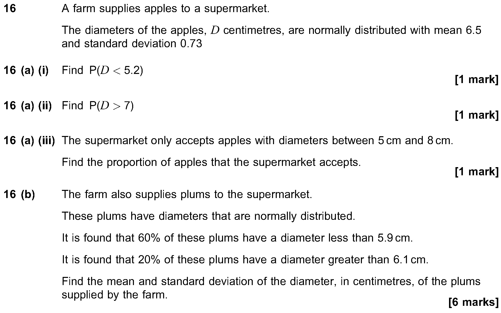
AQA 7357/3 Jun 2023 A2 Exam Q. 16
9 marks in 10:48 min.
Vote:
(0)
(0)
(0)
Request * Pop-Up Working * (0)
Request * Pop-Up Working * (0)
AQA 7357/3 Jun 2022 A2 Exam Q. 11
1 mark in 1:12 min.
Vote:
(0)
(0)
(0)
Request * Pop-Up Working * (0)
Request * Pop-Up Working * (0)
AQA 7357/3 Jun 2022 A2 Exam Q. 18
11 marks in 13:12 min.
Vote:
(0)
(0)
(0)
Request * Pop-Up Working * (0)
Request * Pop-Up Working * (0)
AQA 7357/3 Nov 2021 A2 Exam Q. 18
10 marks in 12:00 min.
Vote:
(0)
(0)
(0)
Request * Pop-Up Working * (0)
Request * Pop-Up Working * (0)
AQA 7357/3 Nov 2020 A2 Exam Q. 17
8 marks in 9:36 min.
Vote:
(0)
(0)
(0)
Request * Pop-Up Working * (0)
Request * Pop-Up Working * (0)
AQA 7357/3 Jun 2019 A2 Exam Q. 17
12 marks in 14:24 min.
Vote:
(0)
(0)
(0)
Request * Pop-Up Working * (0)
Request * Pop-Up Working * (0)
AQA 7357/3 Jun 2018 A2 Exam Q. 16
12 marks in 14:24 min.
Vote:
(0)
(0)
(0)
Request * Pop-Up Working * (0)
Request * Pop-Up Working * (0)
AQA 7357/3 Jun 2017 A2 Sample Exam Q. 13
8 marks in 9:36 min.
Vote:
(0)
(0)
(0)
Request * Pop-Up Working * (0)
Request * Pop-Up Working * (0)
-
Jun 24 A2
P2 Q 9
Jun 24 A2
P2 Q 9
-
Jun 23 A2
P2 Q 11
Jun 23 A2
P2 Q 11
-
Jun 22 A2
P2 Q 9
Jun 22 A2
P2 Q 9
-
Nov 20 A2
P2 Q 11
Nov 20 A2
P2 Q 11
-
Jun 19 A2
P2 Q 9
Jun 19 A2
P2 Q 9
-
Jun 18 A2
P2 Q 8
Jun 18 A2
P2 Q 8
-
Jun 17 A2
P2 Q 7
Jun 17 A2
P2 Q 7
-
Jun 17 A2
P2 Q 8
Jun 17 A2
P2 Q 8
OCR H240/02 Jun 2024 A2 Exam Q. 9
8 marks in 9:36 min.
Vote:
(0)
(0)
(0)
Request * Pop-Up Working * (0)
Request * Pop-Up Working * (0)
OCR H240/02 Jun 2023 A2 Exam Q. 11
9 marks in 10:48 min.
Vote:
(0)
(0)
(0)
Request * Pop-Up Working * (0)
Request * Pop-Up Working * (0)
OCR H240/02 Jun 2022 A2 Exam Q. 9
14 marks in 16:48 min.
Vote:
(0)
(0)
(0)
Request * Pop-Up Working * (0)
Request * Pop-Up Working * (0)
OCR H240/02 Nov 2020 A2 Exam Q. 11
9 marks in 10:48 min.
Vote:
(0)
(0)
(0)
Request * Pop-Up Working * (0)
Request * Pop-Up Working * (0)
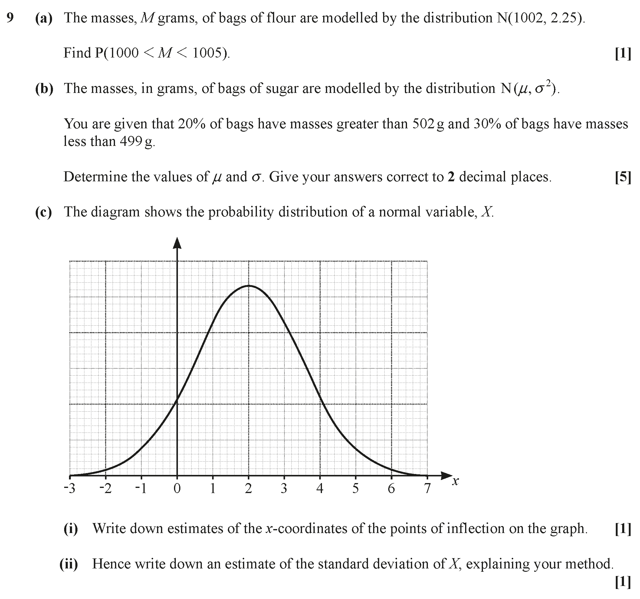
OCR H240/02 Jun 2019 A2 Exam Q. 9
11 marks in 13:12 min.
Vote:
(0)
(0)
(0)
Request * Pop-Up Working * (0)
Request * Pop-Up Working * (0)
OCR H240/02 Jun 2018 A2 Exam Q. 8
8 marks in 9:36 min.
Vote:
(0)
(0)
(0)
Request * Pop-Up Working * (0)
Request * Pop-Up Working * (0)
OCR H240/02 Jun 2017 A2 Sample Exam Q. 7
6 marks in 7:12 min.
Vote:
(0)
(0)
(0)
Request * Pop-Up Working * (0)
Request * Pop-Up Working * (0)
OCR H240/02 Jun 2017 A2 Sample Exam Q. 8
7 marks in 8:24 min.
Vote:
(0)
(0)
(0)
Request * Pop-Up Working * (0)
Request * Pop-Up Working * (0)
-
Jun 22 A2
P2 Q 6
Jun 22 A2
P2 Q 6
-
Jun 22 A2
P2 Q 9
Jun 22 A2
P2 Q 9
-
Nov 21 A2
P2 Q 8
Nov 21 A2
P2 Q 8
-
Nov 20 A2
P2 Q 8 def
Nov 20 A2
P2 Q 8 def
-
Jun 19 A2
P2 Q 15
Jun 19 A2
P2 Q 15
-
Jun 18 A2
P2 Q 10
Jun 18 A2
P2 Q 10
-
Jun 17 A2
P2 Q 6
Jun 17 A2
P2 Q 6
OCR MEI H640/02 Jun 2022 A2 Exam Q. 6
2 marks in 2:24 min.
Vote:
(0)
(0)
(0)
Request * Pop-Up Working * (0)
Request * Pop-Up Working * (0)
OCR MEI H640/02 Jun 2022 A2 Exam Q. 9
9 marks in 10:48 min.
Vote:
(0)
(0)
(0)
Request * Pop-Up Working * (0)
Request * Pop-Up Working * (0)
OCR MEI H640/02 Nov 2021 A2 Exam Q. 8
4 marks in 4:46 min.
Vote:
(0)
(0)
(0)
Request * Pop-Up Working * (0)
Request * Pop-Up Working * (0)
OCR MEI H640/02 Nov 2020 A2 Exam Q. 8 def
6 marks in 7:12 min.
Vote:
(0)
(0)
(0)
Request * Pop-Up Working * (0)
Request * Pop-Up Working * (0)
OCR MEI H640/02 Jun 2019 A2 Exam Q. 15
6 marks in 7:12 min.
Vote:
(0)
(0)
(0)
Request * Pop-Up Working * (0)
Request * Pop-Up Working * (0)
OCR MEI H640/02 Jun 2018 A2 Exam Q. 10
8 marks in 9:36 min.
Vote:
(0)
(0)
(0)
Request * Pop-Up Working * (0)
Request * Pop-Up Working * (0)
OCR MEI H640/02 Jun 2017 A2 Exam Q. 6
4 marks in 4:48 min.
Vote:
(0)
(0)
(0)
Request * Pop-Up Working * (0)
Request * Pop-Up Working * (0)
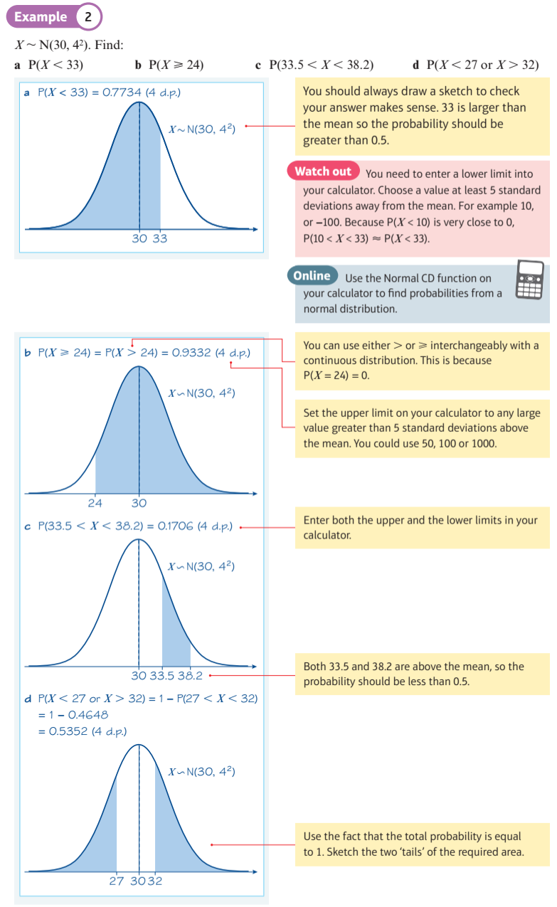
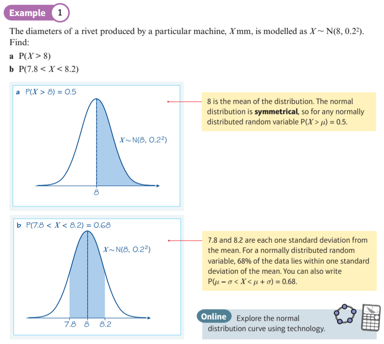
Use the Normal Cumulative Distribution (CD) function
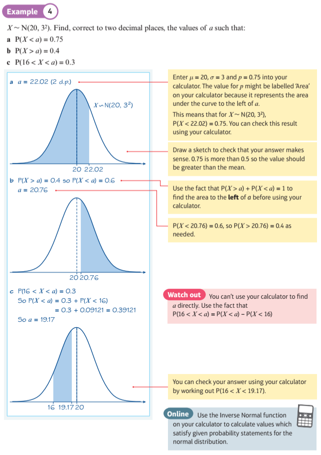
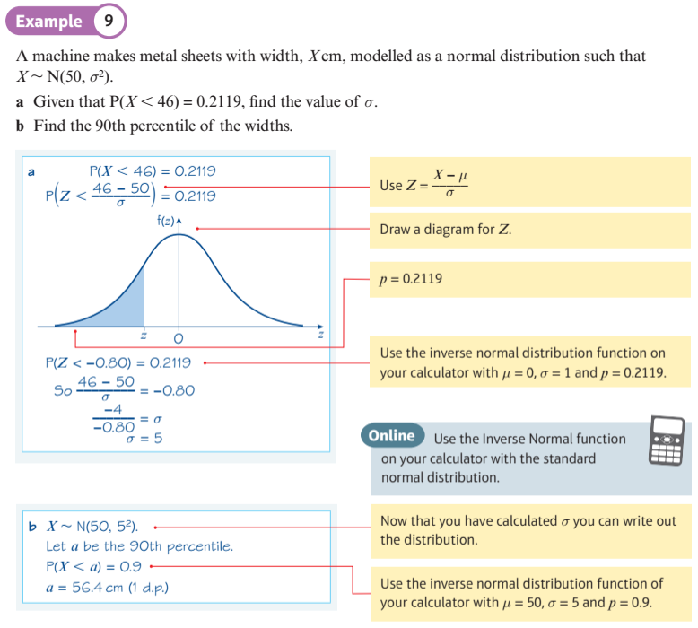
Use the Inverse Normal function
Use the Inverse Normal function with the Standard Normal distribution
Explore the Normal distribution
The Normal Distribution
The normal curve was developed in 1733 by DeMoivre as an approximation to the binomial distribution.
His paper was not discovered until 1924 by Karl Pearson.
Laplace used the normal curve in 1783 to describe the distribution of errors.
Subsequently, Gauss used the normal curve to analyze astronomical data in 1809.
The normal curve is often called the Gaussian distribution.
The term bell-shaped curve is often used in everyday usage.
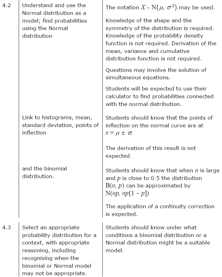
The shape of the normal distribution is determined by two parameters, the mean $\color{blue}{ \mu }$ and the variance $\color{blue}{ { \sigma ^ 2 } }$, and a Normally distributed random variable $\color{blue}{ X }$ is commonly denoted $\color{blue}{ X \sim N(\mu , { \sigma ^ 2 } ) }$.
In the display below you can see the effects of changing the mean and the standard deviation (the square root of the variance).
After selecting "Show Probability", you can also slide the two gliders on the x-axis to see the probability that $\color{blue}{ X }$ falls between them.
Standardising Normal Variables
The 'Standard' Normal distribution is a special case of the Normal distribution with mean, 0 and standard distribution, 1.
The 'Standard' Normal distribution is commonly denoted $\color{green}{ Z \sim N( 0 , { 1 ^ 2 } ) }$.
It would not be possible to provide look-up tables for the probabilities associated with the infinite number of general Normal distributions, but it is possible to provide look-up tables for the Standard Normal distribution. Calculators can also provide probabilities for the Standard Normal distribution. The common practice is to transform, or "standardise", general Normal variables to Standard normal variables, for which look-up tables and calculator functions are available. The transformation may be reversed at the end, if required.
This display allows you to see how the transformation works. You can model a general Normal distribution, $\color{blue}{ X \sim N(\mu , { \sigma ^ 2 } ) }$, and transform it to Y by altering parameters a and b. You should see the required transformation formula when the Y distribution matches the Z distribution.
After selecting "Show Probability", you can also slide the two gliders on the x-axis to see the probability that $\color{blue}{ X }$ falls between them.
Skewed Normal Distribution
The normal curve was developed in 1733 by DeMoivre as an approximation to the binomial distribution.
His paper was not discovered until 1924 by Karl Pearson.
Laplace used the normal curve in 1783 to describe the distribution of errors.
Subsequently, Gauss used the normal curve to analyze astronomical data in 1809.
The normal curve is often called the Gaussian distribution.
The term bell-shaped curve is often used in everyday usage.
The shape of the normal distribution is determined by two parameters, the mean $\color{blue}{ \mu }$ and the variance $\color{blue}{ { \sigma ^ 2 } }$, and a Normally distributed random variable $\color{blue}{ X }$ is commonly denoted $\color{blue}{ X \sim N(\mu , { \sigma ^ 2 } ) }$.
In the display below you can see the effects of changing the mean and the standard deviation (the square root of the variance).
After selecting "Show Probability", you can also slide the two gliders on the x-axis to see the probability that $\color{blue}{ X }$ falls between them.